Want to get started with Polaris? Great! This page will help you do just that.
Prerequisites
You’ll need to have a few things before we can start:
You need Linux or Unix-like environment with Python 3. (Python 2 is not supported.) OS X should work, although we haven’t tried it. (Wondering about Windows? So are we – give it a try and let us know how it works.)
You’ll need to be comfortable installing Python packages – we strongly recommend using virtualenv to create a separate environment for Polaris. If you haven’t done this before, this guide should help you out.
You’ll need to be comfortable with the CLI.
You’ll need a good network connection, so you can download telemetry quickly.
Setting up Polaris
Install Polaris in a virtual environment using pip:
$ mkdir polaris
$ cd polaris
$ python -m venv .venv
$ source .venv/bin/activate
$ pip install --upgrade pip
$ pip install polaris-ml
Note: Various things will break if there is any whitespace in the full path to your virtualenv. Here are some example of paths that will not work:
/home/jdoe/My Development Stuff/polaris/.venv/mnt/C/Jane Doe/dev/polaris/.venv
Instead, use paths without spaces in them:
/home/jdoe/my_development_stuff/polaris/.venv/mnt/c/dev/polaris/.venv
Also, be sure to upgrade pip itself as we’ve shown above – otherwise, you may run into problems installing dependencies.
Advanced: Installing the latest version of Polaris
We push new releases to PyPi as appropriate, but work is continuing on Polaris all the time. If you want to try out the very latest features (and help us with bug reports :grinning:), you can do that like so:
$ git clone https://gitlab.com/librespacefoundation/polaris/polaris.git
$ cd polaris
$ python -m venv .venv
$ source .venv/bin/activate
$ pip install -e .
Running your first analysis: LightSail-2
Now you’re ready to get started on your first analysis. We’ve picked LightSail-2, a mission by The Planetary Society to demonstrate the feasibility of solar sailing, to get started with, as there is a lot of data available.
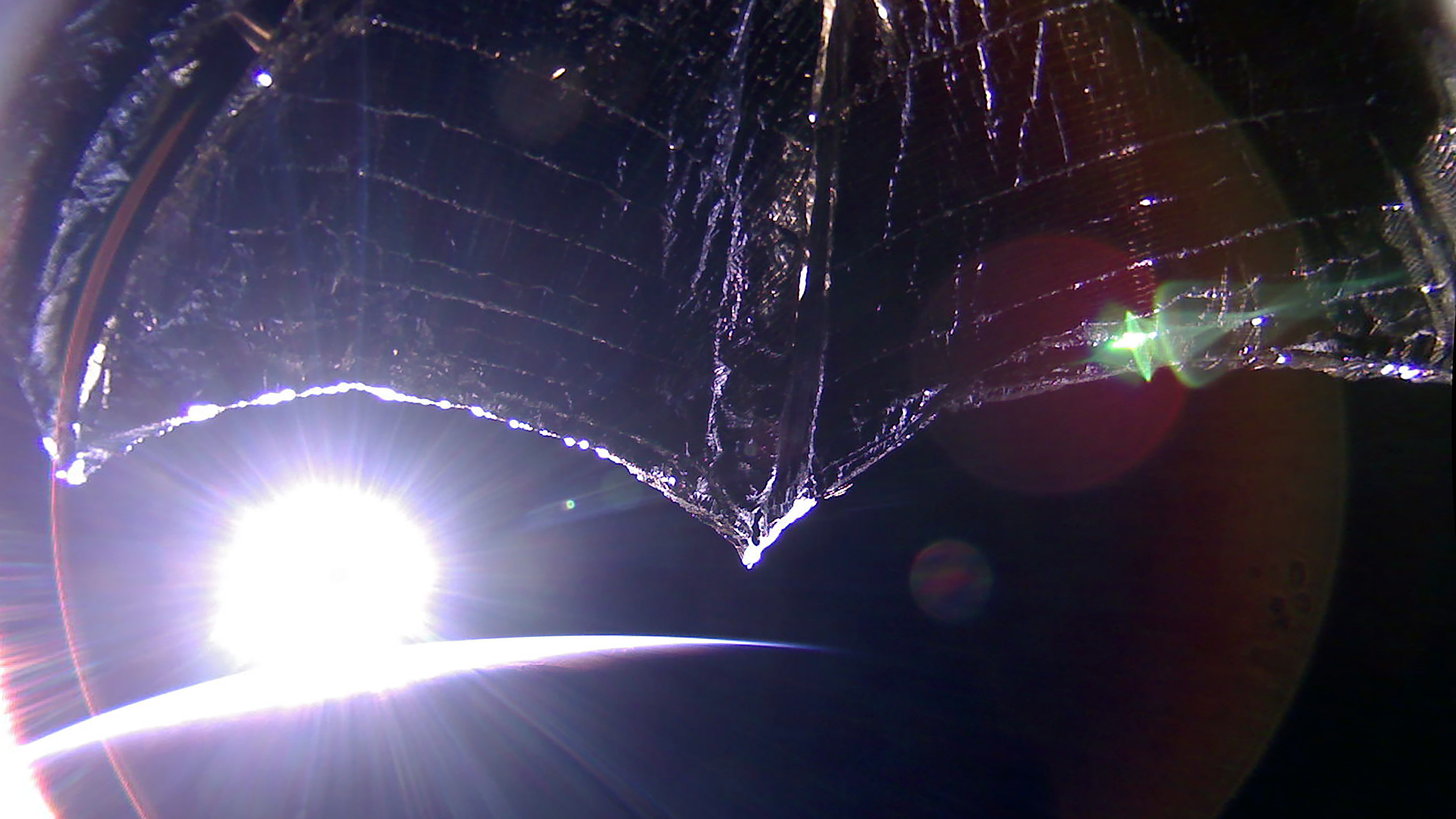
LightSail 2 Orbital Sunrise: The Sun rises over the horizon in this image from LightSail 2 captured on 28 September 2019. The sail appears curved due to the spacecraft’s 185-degree fisheye camera lens. The image has been color corrected and some of the distortion has been removed. Licensed under Creative Commons, BY-CC-NA by The Planetary Society. (Original source.)
Fetching data with polaris fetch
We’ll start by downloading a week’s worth of data from SatNOGS. Run this command:
polaris fetch \
    --start_date 2020-01-21 \
    --end_date 2020-01-28 \
    --cache_dir /tmp/LightSail-2 \
    LightSail-2 \
    /tmp/LightSail2-normalized_frames.json
Some background:
The
--start_dateand--end_datearguments have been picked to favour a shorter download time, at the expense of having a decent amount of data. You can experiment with different dates. (Note: if you create an account at db.satnogs.org, you can see what telemetry they have available, and request data for download – we’ll show you how to import that later on.)The
--cache_dirargument specifies where to cache downloaded data.The
LightSail-2argument specifies a normalizer for the downloaded telemetry. (Note: we’ll show you later on how to analyze data without specifying a normalizer.)The final argument is the path to the output of
polaris fetch: a JSON file with all the normalized data.
The final output will be a JSON file with a list of frames: individual telemetry transmissions from LightSail-2, captured by the SatNOGS network.
Note: If you have installed the latest version of Polaris as detailed above, you will also have space weather data for the time period we’ve fetched. ~~As of September 2020, this has not yet been released to PyPi.~~ Update: The latest PyPi release has space weather support.
Note 2: You can also batch download the frames from satnogs-db (as a csv) and run polaris fetch on that like so:
polaris fetch \
     --import_file ~/Downloads/44420-1363-20200824T065638Z-all.csv \
     --cache_dir /tmp/lightsail2 \
     LightSail-2 \
    /tmp/lightsail2/normalized_frames.json
Let’s take a look at how many frames we have:
$ jq '.frames | length' /tmp/LightSail2-normalized_frames.json
557
557 frames is not a lot; we’d want a great deal more data to do a decent analysis. However, the small sample size makes it quicker to download, and much quicker to analyze.
The next step is to analyze this data.
Analyzing the data with polaris learn
Next, we run polaris learn to analyze the data. This will use the XGBoost library to create a dependency graph for the telemetry we’ve downloaded. Run this command:
polaris learn \
    --force_cpu \
    --output_graph_file /tmp/LightSail2-graph.json \
    /tmp/LightSail2-normalized_frames.json
Some background:
The
--force_cpuoption skips over any attempt to detect or use any GPU you might have. If you have a supported GPU, and your drivers are working, you can try leaving out this argument – it will speed things up immensely.The
--output_graph_fileargument specified where we’d like our dependency graph to be saved. This will be the input for the next step.The final argument is the path to the normalized frame file we produced in the last step with
polaris fetch.
Run times will depend on your hardware and the amount of data fetched. On a 12-core, 2.6GHz i7 laptop, with 16 GB of RAM, polaris learn takes about two minutes.
Visualizing the dependency graph with polaris graph
Finally, we’re ready to look at our dependency graph. Run this command:
polaris viz /tmp/LightSail2-graph.json
This will download some JavaScript dependencies, then open up a web server on your machine. Open your browser and navigate to http://localhost:8080. Here’s what you should be seeing:

Let’s examine the screen:
The name of the satellite,
LightSail-2, is in the top right-hand corner.The search bar is in the top left-hand corner. We’ll come back to this in a moment.
The circles in the middle are the nodes of the dependency graph. Each one represents an element of telemetry. The name of that element is displayed beside it.
The lines connecting the nodes represent connections between those nodes – that is, the model constructed by polaris learn has these two nodes varying in concert with each other.
You can navigate this graph:
The scroll wheel on your mouse will zoom in or out.
If you click-and-drag on empty space with your left mouse button, you can rotate the graph.
If you click-and-drag on a node with your left mouse button, you can drag that node around.
If you click-and-drag with your middle mouse button, you can drag the whole graph around.
If you left-click on a particular node, you will zoom into that node.
When you’re zoomed into a node, you’ll see the lines connecting it to other nodes (unless it’s a node that doesn’t have a connection to anything else!). You’ll also see dots moving along those lines. Those dots represent the strength of the connection: a faster-moving dot means a stronger connection.
Zoom back out again. Click on the search bar, and type py_tmp. You should see a list of node names come up as you type; you should end up with just py_tmp:py_tmp/0 as a candidate. Click on that, and you should zoom into that node.
Zoom back out again. Click on the search bar, and type tmp. Pause for a moment, and scroll through the list of nodes: these are all the nodes that have tmp somewhere in their name. Now hit Ctrl-enter (that is, the control and enter key at the same time). You should now see all of those nodes – the ones with tmp in their name – higlighted in the same colour.
Click on the search bar again, and go through that same process with each of the following:
magcampwr
Make sure you hit Ctrl-enter after each one, but this time hit it a few times. Note how each group is being highlighted in different colours, changing each time you hit Ctrl-enter. This allows you to pick colours that work for you.
Looking at the display, we see a number of different things:
There are different collections of nodes, each with their own colours.
The groups of nodes have similar names; we can guess that they probably have similar functions.
The groups are clustered in different ways, showing connections between these groups; this suggests that our model has found connections between different groups of functions.
The satellite operator, at this point, will be able to examine the graph with an eye toward finding connections between elements that may not have been noticed previously.
Conclusion
Here we’ve taken you through the basics of the Polaris workflow:
we’ve picked a satellite to work with;
we’ve downloaded and normalized data captured by the SatNOGS network from that satellite;
we’ve created a model of the connections between the telemetry elements;
we’ve used that model to create a dependency graph;
and we’ve displayed and examined the visualization of that graph.
Next Steps
How to work with space weather data
Using Polaris without a normalizer
Downloading all the data SatNOGS has captured for a particular satellite